Time complexity stands as a pivotal pillar in algorithmic analysis, shedding light on how an algorithm's runtime escalates with the magnitude of its input. It furnishes us with invaluable insights into the efficiency of algorithms, facilitating the judicious selection of approaches tailored to diverse data sizes. This article delves deeply into the intricacies of time complexity and its diverse notations, encompassing Big O, Big Omega, Theta, Little O, and Little Omega. By the end, you'll possess a comprehensive comprehension of algorithmic efficiency.

Time Complexity in Detail:

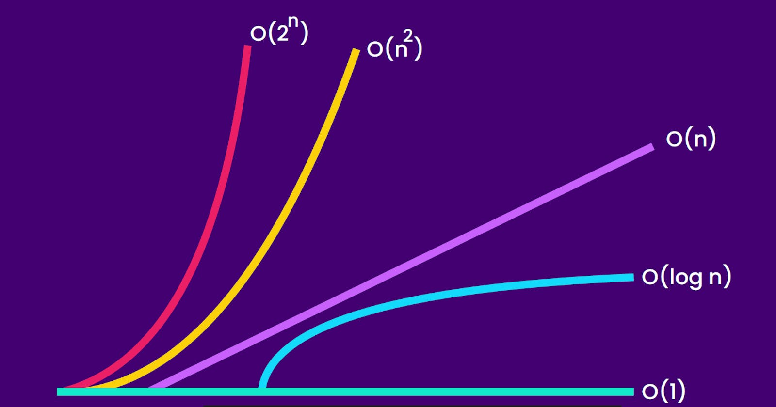
1. Time Complexity Overview: Time complexity serves as a mathematical function that unfurls the runtime's growth concerning the enlarging input. It stands as the compass to gauge algorithmic efficiency and navigate the terrain of algorithm selection. For example, in the realm of linear search versus binary search, binary search triumphs with aplomb when dealing with substantial datasets. Time complexities are symbolized as O(N), O(log N), and O(1) for linear search, binary search, and constant search, respectively, with their time implications: O(1) < O(log N) < O(N).

2. Core Considerations in Complexity Analysis:

   • Worst-Case Analysis: Predominantly, time complexity analysis homes in on the worst-case scenario, thereby establishing an upper time boundary.

   • Scalability for Large or Infinite Data: The analysis unfolds against the backdrop of substantial or infinite data sets, assuring the algorithm's efficiency at all scales.

   • Constant Oversight: Constants are omitted in complexity analysis because they exert a minuscule influence on actual runtime. Focus fixates solely on the interplay between temporal expansion and data augmentation.

3. Abandoning Less Dominant Terms: In the realm of time complexity, the marginal players, or less dominant terms, are benched. Instead, all attention zeroes in on the term sporting the highest exponent. This approach is embraced due to the inconsequential nature of the marginal contributors to execution time.

4. Exemplifying Time Complexity: Ponder an equation sporting time complexity: O(3N^3 + 4N^2 + 5N + 6). Constants and less dominant terms, like N^2 and N, are cast aside, and the time complexity condenses to O(N^3).

Notations in Algorithm Analysis:

Big O Notation:

• Definition: Big O notation dons the mantle of an upper bound, encapsulating the time complexity of an algorithm. It signifies that the algorithm's runtime will not transcend the ceiling established by Big O.

• Mathematical Expression: Big O notation assumes the form f(N) = O(g(N)), where, as N stretches to infinity, the quotient f(N)/g(N) remains finite and does not ascend into the realm of infinity.

• Illustrative Instance: Envision a sorting algorithm, its time complexity an O(N^2. In this scenario, the algorithm's runtime won't surpass the quadratic proportionality to the input size, ensuring efficiency for large datasets.

Big Omega Notation:

• Definition: Big Omega notation unravels the floor for an algorithm's time complexity. If an algorithm brandishes a Big Omega label of N^3, it guarantees that the algorithm will endure at least the specified duration and can stretch beyond it.

• Mathematical Representation: Big Omega notation transpires as f(N) = Ω(g(N)), signifying that, as N trends towards infinity, the ratio f(N)/g(N) holds onto a finite form and doesn't plummet into the depths of infinity.

• Demonstrative Example: Suppose an algorithm beckons with a time complexity of Ω(N^2). Here, the algorithm assures a performance that never stoops below the quadratic relationship with the input size, rendering it a worthy choice for voluminous datasets.

Theta Notation:

• Definition: Theta notation strikes a harmonious balance between Big O and Big Omega, providing both an upper and lower bound for an algorithm's time complexity. It serves as a tight-fitting jacket, encapsulating the algorithm's temporal behaviors.

• Mathematical Expression: Theta notation materializes as f(N) = Θ(g(N)), symbolizing that as N advances to infinity, f(N)/g(N) preserves a finite value.

Little O Notation:

• Definition: Little O notation, a kin to Big O, delivers an upper bound but with an exclusive clause—here, the algorithm's runtime is strictly less than the bound. It defines a level of efficiency that won't be reached, even as input size escalates.

• Mathematical Formulation: Little O notation assumes the form f(N) = o(g(N)), where, with N heading towards infinity, f(N)/g(N) approaches zero.

Little Omega Notation:

• Definition: Little Omega notation, akin to Big Omega, furnishes a lower bound, but with a particular nuance—the algorithm's runtime surpasses the bound, ensuring a degree of inefficiency.

• Mathematical Representation: Little Omega notation appears as f(N) = ω(g(N)), suggesting that as N marches towards infinity, f(N)/g(N) never dwindles to zero.

Comparing Notations:

• Big O vs. Little O: Big O offers an upper bound, signifying that an algorithm will not be less efficient than what is described. In contrast, Little O stipulates that an algorithm will always be more efficient, ensuring a superior performance than what is bounded.

• Big Omega vs. Little Omega: Big Omega serves as a lower bound, guaranteeing a minimum efficiency level. On the other hand, Little Omega specifies that an algorithm can perform even more efficiently, transcending the bound established.

In conclusion, the exploration of time complexity and its diverse notations equips us to make informed decisions in algorithm selection. By understanding these notations and their distinctions, we gain a powerful toolkit for assessing efficiency and scalability, empowering us to choose the most fitting algorithms for a multitude of computational tasks.